
Morphological optimization of Neural Networks
How to pick the optimal model for the efficiency of training algorithm
Reading Time: 7 minutes
Among the Machine Learning models, the one of the Neural Networks is one of those with the highest computational cost. By its nature, the neural network lends itself well to simulate multiple real cases and finds application in many areas. However, its “slowness” is often the cause of its exclusion to act as a model solving many problems.
To solve this problem we can work in two directions: space and time. Leaving aside the first aspect, now widely treated with quantum computers, in the modelling phase we can however intervene on the resource “time” through methods of optimization of algorithms.
Given the breadth and complexity of the subject, in this article we will therefore focus on how to intervene on the architecture of the model in order to reduce the amount of time needed for computation and improve the efficiency of the training algorithm of the network.
Goals
Most of the time we talk about the optimization of a neural network we refer to the data training phase only. It is therefore linked to the network instructor’s experience in finding the right ratio for the size of the training set. Instead, we want to focus on the structure of the network and analyze optimization methods related to its architecture in relation to the degree of precision that is attempted to obtain.
In this article we will use a neural network with few layers and few neurons and with simple exercises related only to supervised learning given the didactic purpose of the article itself and to focus on optimization rather than in the network itself. The important thing is the concept, to understand the message that we want to communicate that is to obtain an analytical vision of the models of AI to be able to intervene where and how each of us is able according to their own resources.
So let’s get started!
The Neural Network
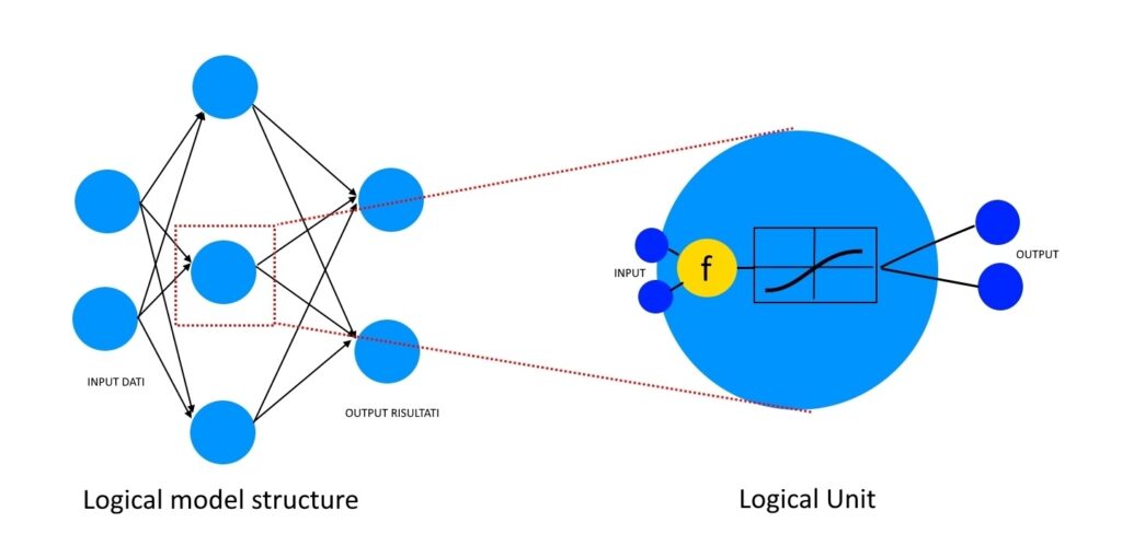
Artificial networks simulate the functioning of biological networks by replicating their functioning scheme: neurons receive input data, process them and are able to send output information to other neurons. The node is the elementary unit of calculation that simulates the neuron and transforms a data vector input x = (x1; x2; … ; xn) in an output y(x) through a function g, usually non-linear, called function of activation of the neuron.
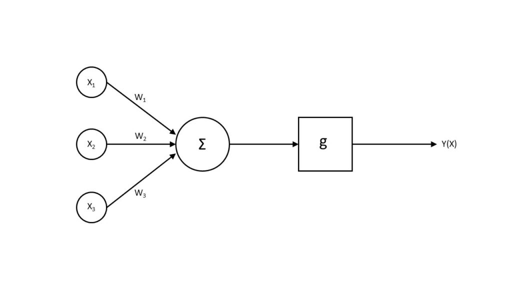
In the analogy with the biological brain, each input value xi is multiplied by a weight wi that simulates the synaptic connection for the determination of the correct outputs. Therefore, the weighted algebraic sum of the inputs is passed on to the activation function g at the input. This is compared with a “threshold” value ɵ. The neuron is activated only if the weighted sum of the inputs exceeds the threshold value ɵ:
y(x) = g (∑ – ɵ)
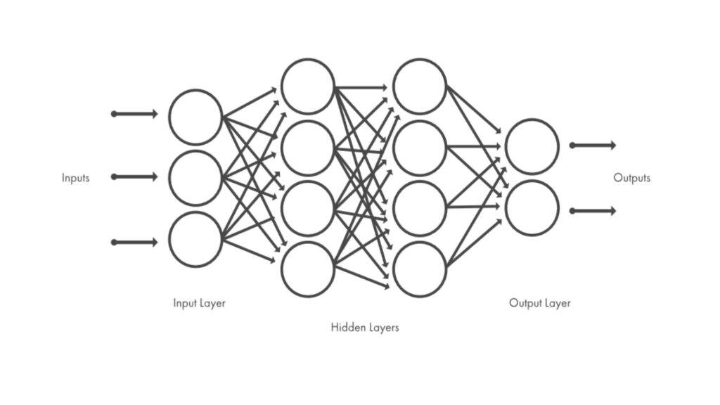
The number of nodes, their arrangement within the network and the orientation of the connections determine the type of neural network. They can be distinguished according to the synaptic connection, which can be described by differential equations or polynomial functions, or according to their morphological structure. Then we can see networks described by oriented graphs or by multilayer networks.
Further distinctions can be introduced in relation to the training methodology used. The training of the network consists in making elaborate a sufficiently high number of input-elaboration-output cycles, with inputs that are part of the training set, in order to make the network able to generalize, that is to supply correct outputs associated to new inputs. The type of training received decrees the known classification on supervised, unsupervised and reinforcement learning.
Network optimization
Supervised learning involves providing the network with a set of inputs to which correspond known outputs (training sets) through successive cycles. At each cycle they are analyzed and re-elaborated by the network in order to learn the nexus that unites them.
Normally the approach that is followed is to correct the weights to get better answers: we increase the weights that determine the correct outputs and decrease those that generate invalid values. Most of the texts on the neural networks deal with the argument of the right value of the weights.
Our study instead starts from the assumption that training is given as a matter of fact, both in terms of the number of known data and expected results, and focuses instead on varying the number of neurons within the network in order to lower the execution time of the supervised algorithm.
As mentioned in the introduction to the article, we work with simple examples so as not to complicate the treatment and succeed in reaching our goal first. Therefore, we will used a network with only one hidden layer and with 2 inputs and 1 output. This basic structure is more than enough to do our tests. The calculation that our network will have to learn to do is the simplest possible one, a sum.
Once the inputs and outputs are fixed, our optimization work consists in selecting the right number of neurons in the hidden layer. To do this we train the network to make our sum first with an architecture that includes 6 neurons in the hidden layer, then 3. Let’s compare the results obtained and try to reach a plausible conclusion for our morphological optimization
Training
The supervised learning mechanism uses Error Back-Propagation, a training algorithm that aims to find the optimal weights of the network through an iterative evaluation procedure. After a random initialization of the weights, iteratively couples of input-outputs, being part of a predefined set of data, are provided to the model and the appropriate updates of the weights are carried out at each cycle. The iteration stops when the absolute minimum of the distance between the desired outputs and the corresponding outputs calculated by the model is obtained, that is the minimum of the following cost function
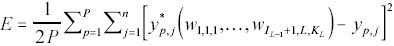
where:
P is the number of input-output pairs in the defined data set,
n is the size of the output vector calculated by the model
The modification of the weights is obtained therefore retropropagating the value assumed by the function of cost from the layer of output, through the hidden layers, until the initial layer of input. From here it is deduced that the computational cost of the training function depends on the number of neurons belonging to the layers of the network. For the simplification wanted to give to our article, our attention will be on the number of neurons present in the hidden layer.
The transfer functions considered are:
- logistic function for the nodes of the hidden layer
- linear function for the output node
Let’s remember the equation of the logistic function or Sigmoid:
O = 1/(1+exp(-I))
where
O = neuron output
I = sum of neuron inputs
Results
We are going to operate two different trainings whose settings are as follows:
First
NETWORK SETTINGS
N. Input 2
N. Neurones (hidden layer) 6
N. Output 1
Transfer function Sigmoid
Second
NETWORK SETTINGS
N. Input 2
N. Neurones (hidden layer) 3
N. Output 1
Transfer function Sigmoid
Since we do not want to intervene in the optimization of the training side, the settings will be common to the two trainings and will remain so constantly:
TRAINING SETTINGS
Max Error 0,02
Training rate 0,3
We do our training. We observe that the calculation time is inversely proportional to the error of the cycles. We obtain short times, in the order of a few seconds, at the expense, however, of propagation errors that are too far from the permitted value in the setting phase (0,02).
We report only the most significant results:
Training N.1 (6 neurones)
Number of cycles 61892
Error cycle 0,029
Second employees 565
Training N.2 (3 neurones)
Number of cycles 60651
Error cycles 0,029
Second employees 261
At a first analysis we can say that halving the number of neurons in the inner layer halves the calculation time of the training algorithm with the same goodness of the model (the error remains constant over the time).
Conclusion
By doing all the necessary tests in the laboratory, we arrived at a very important observation: the reduction of neurons within the hidden layers of a multilayer neural network allows to increase the calculation speed of the model of 53.8% compared to a non-optimized network thus increasing the performance of the overall model.
The construction of the correct architecture of the neural network, through a considered choice of layers and neurons, allows a greater efficiency of the algorithms and, consequently, a greater adaptability of the network itself to be really used in real cases.
Good modeling, everyone!
This article was written by Ph. D. Donata Petrelli for the Ms. AI Expert blog and is available in its original form at this address:
https://www.nemesventures.com/post/morphological-optimization-of-neural-networks