Gaussian distribution and shoe comfort index

… when statistical data analysis disproves our assumptions!

Reading Time: 6 minutes

Post published on 29/10/2020 by Donata Petrelli and released with licenza CC BY-NC-ND 3.0 IT (Creative Common – Attribuzione – Non commerciale – Non opere derivate 3.0 Italia)

It’s common opinion that high heels are sexy but very uncomfortable …

We can also agree on the first point, that shoes with high heels are fascinating, but is it also true that they are uncomfortable?

Not always what seems an obvious answer is also scientifically true. In this regard we are helped by statistical analysis that allows us to evaluate a given hypothesis on a sample of real data and help us to find a solution to decision-making problems.

One of the basic techniques is the Gauss distribution, also called the “Normal” distribution since it’s normally used as a first approximation to describe the behavior of real causal values that tend to concentrate around a single value, the average.

The use of the Gaussian model for data analysis is so popular that I thought to talk about it in this article. It is in fact applied in many fields, from medicine, sociology, economics and finance … up to the evaluation of the comfort of our shoes 🙂

If you want to know more … please continue reading.

Average and Standard Deviation

To begin with we must start from the basics. The statistical analysis, including the Gauss distribution, is based on two fundamental concepts: average and standard deviation.

The concept of mean is so well established that we also use it for simple daily analysis. For example, we express with an average cost the food expenditure that we incur monthly to get an idea of our needs, taking into account that there are months when consumption is higher and others when it is lower. The average is the statistical tool that describes the behavior of a certain phenomenon that varies over time by expressing it with a single number.

The arithmetic mean is the sum of a collection of numbers divided by the count of numbers in the collection.

Its mathematical formula is:

$\inline \mu = \sum_{i=1}^{N}xi/N$

µ = (x₁ + x₂ + … + x_N) / N

where

x_i is the i-th value of collection
N is the count of numbers in the collection

In Excel you use the AVERAGE function. Its syntax is:

AVERAGE(number1, [number2], …)

where

Number1 is the first number, cell reference, or range for which you want the average. Required
Number2, … Additional numbers, cell references or ranges for which you want the average, up to a maximum of 255. Optional.

Often a single number is not enough to summarize the behavior of a dynamic phenomenon that evolves over time. It is necessary to know another aspect that describes its variability, that is the tendency to manifest itself in different and distant ways over time.

To measure this variability there is another very important statistical indicator, of which we make a habitual use often unconsciously, the Standard Deviation. This indicator measures the propensity of a certain phenomenon to ‘move away’ from its reference value, the average in our case.

Its mathematical formula is:

$\inline \sigma = \sqrt{1/N \sum_{i=1}^{N}(xi - \mu )^{2}}$

where

N is the count of data in the collection or population size
μ is the mean of the population.

The Standard Deviation can be easily calculated in Excel thanks to the STDEV.S function.

Its syntax is:

STDEV.S(number1,[number2],…)

where

Number1 is the first number argument corresponding to a sample of a population. You can also use a single array or a reference to an array instead of arguments separated by commas. Required
Number2, … Number arguments 2 to 254 corresponding to a sample of a population. You can also use a single array or a reference to an array instead of arguments separated by commas. Optional.

Thanks to these two indicators, mean value and standard deviation, we can get an idea of the behavior of the phenomenon. The first one tells us which value tends to assume in time, the second one how much is variable around it.

If the standard deviation (σ) is a large measure, the distribution values are dispersed with respect to their average reference value. Conversely, if the standard deviation is small, the values are concentrated near the mean.

Normal distribution

Very often it happens that the values are distributed in such a way that their density is increasing as you reach a central value, the average, here they touch the maximum point, then begin to decrease again to zero. In this case the values follow the normal distribution according to the typical bell curve.

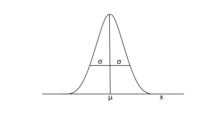
Article-Gauss-Figure-1 — Figure 1 – Normal Distribution

These distributions are characterized by two aspects:

height
width

This typical bell shape depends on the value of the variance, i.e. their variability. This means that distributions with strong variability have a Gaussian representation with the bell of greater amplitude than those with less variability.

The normal distribution is a function of probability, so the area under the curve is always equal to 1. For this reason, if its width varies, the height must necessarily vary. If σ increases the height decreases and vice versa.

The other aspect to consider is the position of the bell in the horizontal axis. This depends on the mean value μ: the larger it is, the more it will be shifted to the right of the x-axis.

The following figure shows the differences:

Article-Gauss-Figure-2 — Figure 2 – Different bell curves

From the curve we can already guess the type of probability distribution.

Gaussian function

What is behind all this? … a Gaussian!

The formula underlying the Gauss model is a function that depends exclusively on the two parameters μ and σ. The mathematical function is:

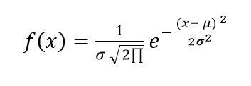
where

μ the mean of the values
σ the standard deviation of the values
σ² the Variance

The variance (σ2) is a measure of how far each value in the data set is from the mean. It’ s defined as the average of the squared differences from the Mean.

In Excel, the function that returns the normal distribution for the specified average and standard deviation is NORM.DIST function. The NORM.DIST function syntax is:

NORM.DIST(x,mean,standard_dev,cumulative)

where

X is the value for which you want the distribution. Required.
Mean is the arithmetic mean of the distribution. Required.
Standard_dev is the standard deviation of the distribution. Required
Cumulative A logical value that determines the form of the function. If cumulative is TRUE, NORM.DIST returns the cumulative distribution function; if FALSE, it returns the probability density function. Required

The solution via Gauss

Once we understand how Gauss’s probability distribution works, we return to our case. I have noticed that I can wear shoes with 12 heels more comfortably than others with lower heels. Why?

I thought that probably the comfort is not given by the height of the heel but by another parameter. So I considered the distance between the sole and the heel. I took these measurements in all my shoes, indistinctly from the heel height, and reported them on an Excel spreadsheet.

Then I calculated the Average, the Standard Deviation and the Normal Distribution for them using the Excel functions described above and I obtained the following result:

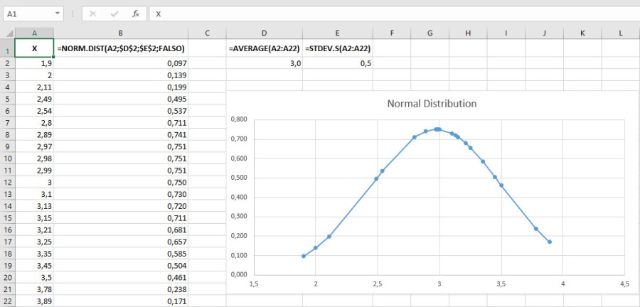
Article-Gauss-Figure-3 — Figure 3 – Normal Distribution of measures

Surprise! The statistical analysis of the shoes I usually wear shows that the difference is not the height of the heel, but the distance between the sole and the heel!

The ideal distance is 3 centimeters which represent the comfort index of the shoes. Even half a centimeter less is enough that the shoe will be extremely uncomfortable.

The physical explanation of the numerical result is that a smaller distance between sole and heel means a greater inclination of the shoe and therefore the greater the weight that the toes will have to bear

Article-Gauss-Figure_4 — Figure 4 – Source www.shefinds.com

Conclusion

When we have to make considerations and based on them make decisions, the right thing to do is an initial statistical data analysis.

In this article we have dealt with one of the most powerful statistical analysis tools, the Gauss distribution, and we did it through Excel because it is the most popular and easy to use tool for everyone.

The analysis of Gaussian has an enormous importance. The general rule is that 68.2% of the data, of a normal distribution, falls in a precise range that has center in the mean value μ and radius equal to σ.

So if, for example, you have to buy shoes online, do not focus on the heel (thinking that if high then they will be uncomfortable) but it is better to choose those with a distance of about 3 cm between the heel and the sole because most of the comfortable ones fall within this range 🙂

The Gaussian distribution has a very wide application in different fields. Which ones come to mind?

If you want to answer … please go here