Timeline with PivotTable

Advanced Excel techniques for time series

Published on 18/02/2021 by Donata Petrelli

Reading Time: 6 minutes

Are you familiar with an Escher painting?

Depending on how we look at it, different images are shown. Often it is a representation of the same object but from different perspectives. So it happens with data. We often deal with tables of data and don’t know how to extract information from them. Like Escher’s paintings, the trick is to find the right perspective!

To conduct such analysis there are different techniques and different tools. Excel PivotTables are a very powerful and flexible tool for analyzing data dynamically. They form the basis of excellent Business Intelligence without having to bother with much more complex programs.

Very often, however, they are used without taking advantage of all its innumerable potentialities. In this article we’ll see how to use one of these useful functions, surely one of the least known, but extremely useful: Timeline.

Timeline is used to add further control over PivotTables where dates are present and will allow you to have greater control over data being analyzed despite its extreme ease of implementation.

Data

It frequently happens to have to analyze data where they are present, in addition to the classes numbers and alphanumeric characters, even the dates that represent days, weeks, hours, months, etc..

We make a practical example starting from a hypothetical table like that one of Figure 1

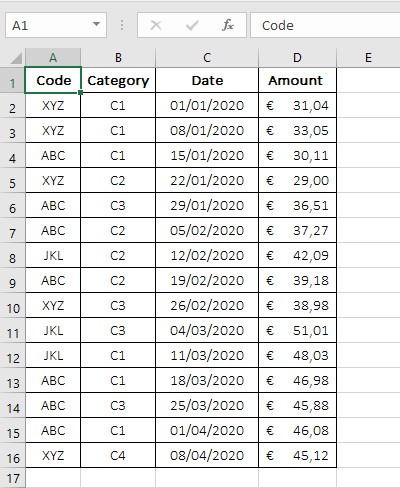
This example is intentionally created generic in order to better explain the concept, without analyzing a specific case that could be misleading. I suggest therefore to adapt the table using data of useful situations in your context or, perhaps, with real data.

PivotTable

Now select all data and create a PivotTable by ” Insert /PivotTable”. The usual Pivot Table creation panel will appear where we will specify that we want to place the PivotTable in the existing sheet and more precisely starting from cell G1 as indicated in Figure 2.

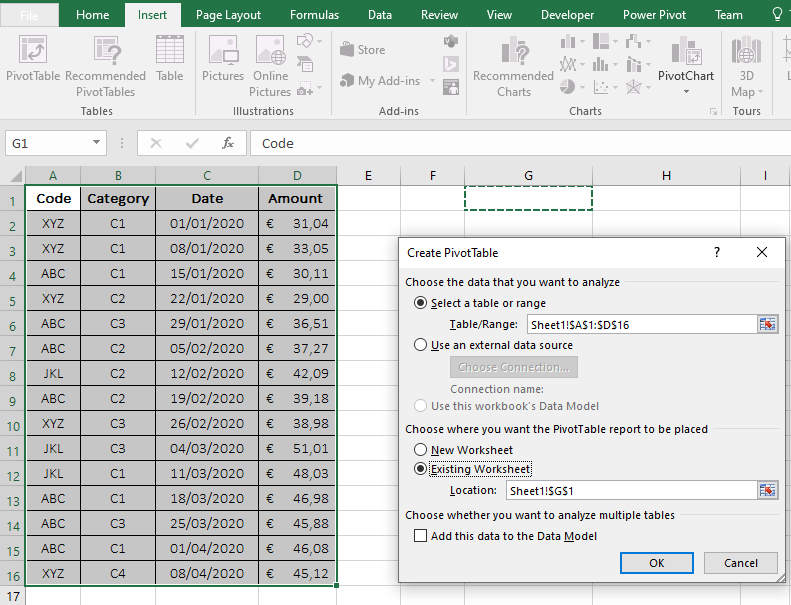
Press OK button.

We must select the fields to be inserted in the respective sections. In our case we will insert CODE in columns, CATEGORY in rows and AMOUNT in values, leaving out, at least for the moment, Date. The result of this operation is shown in Figure 3

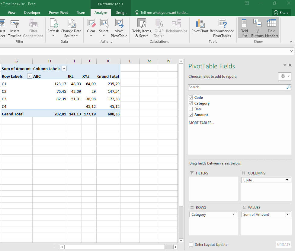
This is the classic and basic PivotTable that we can make in a very simple way.

Date type fields

From here on we will see how to treat the Date field present in the third column of the data source table and listed among the available fields of the PivotTables.

The first thing we can do is add the date field to the filter section. We have added it to the filter field because adding it to the rows or columns section would not be very useful except in very specific cases.

The addition of this field in the filters section enables a new element in the table with which we can filter the Pivot Table data according to the section. This is a filter and behaves as such like all other filters in Excel.

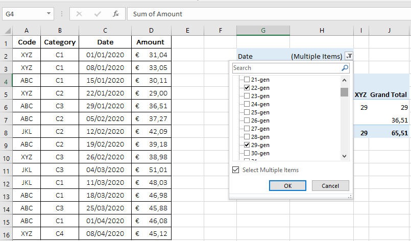
As a basic setting we have all the fields selected, but if we click on the arrow of the filter, a list of dates will appear that we can select/deselect as we wish so as to analyze the data in certain interesting cases. We can select a single date or more dates by selecting the item “Select Multiple Items” as you can see from Figure 4.

The use of filters, in this case with the Data field, certainly makes data analysis more flexible with even more specific parameterizations. In this case, however, it is not a very convenient method for a dynamic analysis as we would like.

Timeline

To overcome this inconvenience we are going to discover a new tool created especially for the advanced management of Dates in PivotTables. This tool is called Timelines

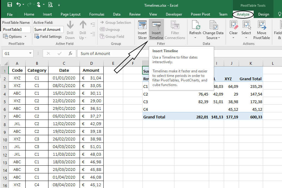
Select PivotTable in the sheet and automatically all the tools related to it will be activated in the menu bar. From the “Analyze” menu, click on “Insert Timeline” in the Filter section, as in Figure 5.

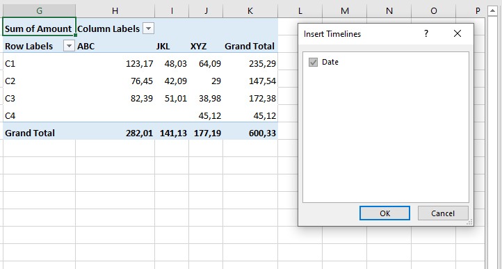
By clicking on the “Insert Timeline” icon, a dialog box will appear asking which field to use. In our case only the Date field appears and must be selected after which we must press the OK button as shown in Figure 6.

Excel automatically analyzes the single fields present in the list of fields of the table looking for those fields that have a precise date type format. Therefore it is advisable, as a general rule, to check the cells so that they are formatted correctly. If the format is not correct you might not see the field you are interested in, while, more complex, if there are only a few fields in the column that are not formatted correctly you might see the column but have inconsistencies in the results.

If everything has been done regularly you’ll see the result of the operation as in Figure 7

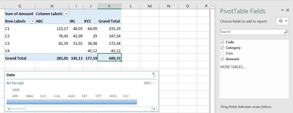
In fact a Timeline is nothing but a specific filter on a Date field with which you can interact in a visual way through a simplified interface.

As soon as it is inserted, for initial setting, we are faced with a time span ranging from the minimum date to the maximum date in the column containing the dates. All dates are selected. But if we go to click on individual elements in the Timeline we will get a selection of only the selected month or months. The data in PivotTable will be automatically recalculated taking into account the data included in the selected months.

That’s it! Simple … right?

Customize

Let’s go further and refine the parameters of our Timeline

What Excel proposes on the Timeline depends on the type of data stored in the column containing the dates. Without going into detail about all possible cases and their combinations, we will limit ourselves to the analysis of what we have created with our table and data we have available.

let’s see how to improve our analysis by interacting with a parameter in the Timeline panel.

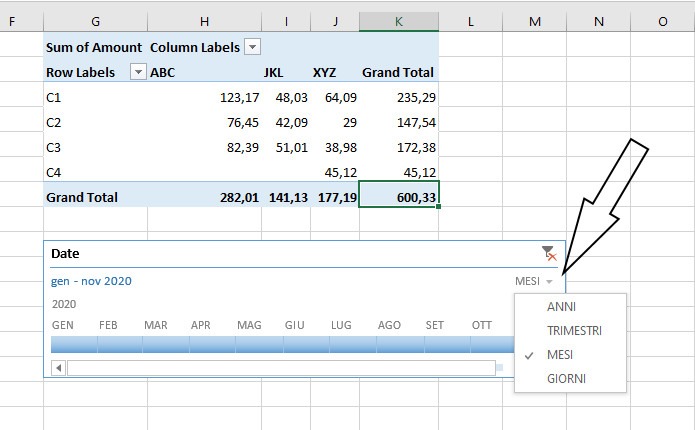
In Figure 8 you can see that there is a selection menu in the top right corner. It is set automatically by Excel based on the analysis of the data available in the table but we can modify it.  In our case it is set to MONTHS and indicates a filter based on months. We can select other types of filter such as YEARS, QUARTERS or DAYS, adapting it to our needs at the moment.

Conclusion

In addition to being used in advanced analysis processes, such as classifications, calculations and data summarization, PivotTables allow you to quickly draw up reports of the analyses done, thanks to which you can make comparisons, find patterns and data trends.

Here we have seen how temporal analyses are facilitated by the use of the Timelines filter. It is therefore a powerful data analysis tool but, at the same time, easy to use and, therefore, suitable for everyone, even for non-technical or programming experts, but who still need to make analysis for their business.

If you find this article useful and would like to discover other tricks for data analysis I suggest you to subscribe to my newsletter to receive all the news and updates.

Thanks!