What is the best time to launch a marketing campaign?

Skewness reveals this to us!

Published by Donata Petrelli on 13/05/2021

Image credits by Elio Santos

Reading Time: 6 minutes

From the visits to the e-commerce site to the number of sales in the last year, from the enrolments to the online courses to the results of the final tests … data we collect tells a story. As a story has its moral, data wants to convey information. Knowing how to read and understand the behavior of data means finding this information. From the graphical analysis of a distribution it is already possible to understand the character of data.

In the article “Gaussian distribution and shoe comfort index” I talked about the Gauss or “Normal” distribution as a first approximation to describe the behavior of values that tend to concentrate around a single value and how this data can be synthesized through indices. It is precisely a deeper study of this distribution that leads us to understand which index succeeds in representing the central tendency of the data and adopt it as a reference value for our business decisions.

From this point of view it is therefore useful to study the “shape” of this normal distribution because while in theory we are dealing with a curve symmetrical with respect to its mean, in reality it is almost never so. Small shifts make the curves instead asymmetrical with respect to the central value. This study is possible thanks to the shape parameters.

In this article we want to consider skewness. Understanding what it is, what it is for, and how it is calculated allows us to immediately benefit from shape analysis to make optimal decisions in the context described by data.

Skewness

Skewness measures the absence of symmetry of a frequency distribution.

A data distribution is symmetric if there is a value (the mean) that divides the distribution into two parts, with the elements of each part symmetrical of the corresponding elements of the other part. If this does not occur, the distribution is asymmetric.

Meaning of Skewness

Two types of Skewness can occur in a distribution of values:

Right-skewed: when the values that are furthest from the mean are the highest and are therefore to the right of the central values (Figure 1)
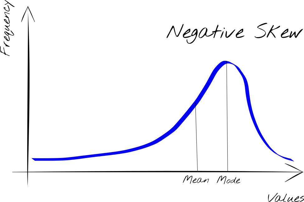
Left-skewed: when the extreme values, those furthest from the average, are the least (Figure 2)

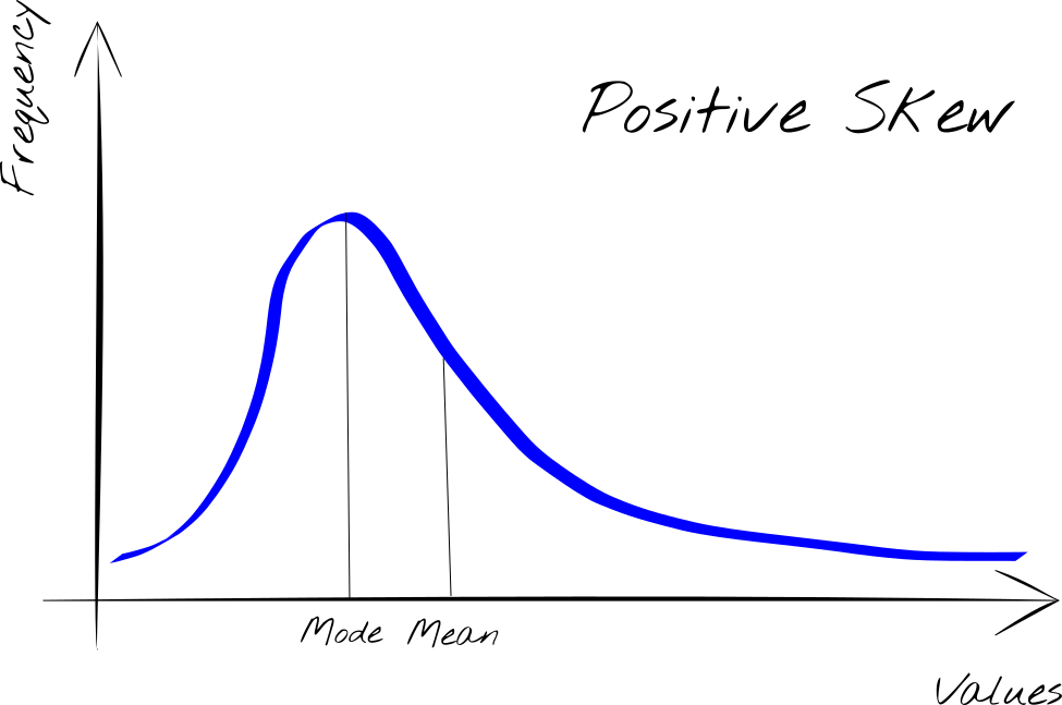
The positive skew reveals skewed to the right.

The negative skew reveals skewed to the left.

Why it matters

The interpretation of the Skewness reveals an important aspect of the distribution of the data. In these cases, the values do not tend to position themselves around the mean value, as happens for the normal distribution, because the mean is affected by the presence of a longer tail (right or left).

In this case then our distribution of values will be concentrated around another value, the one that is observed with greater frequency. This value to take into account for our analysis is the Mode.

Although we are accustomed to consider the Mean as a reference parameter for the description of data, in the case of a skewness of the curve, the Mean is no longer sufficient to summarize the data, but it is preferable to take into consideration the Mode.

How to calculate Skewness

Referring back to the previous description, the simplest method to calculate the skewness is the one that takes into account the Mean and Mode. Thanks to these two values we can calculate the skewness in an absolute way through the difference (d) between the Mean and Mode:

d = Mean – Mode

where

if d = 0, curve is symmetrical
if d > 0, curve has positive skew (or right)
if d < 0, curve has negative skew (or left)

Pearson’s first skewness coefficient

We often find ourselves comparing different distributions of data. In this case we cannot use an absolute value because it is related to the size of the measures. To compare the degrees of skewness of different distributions we must instead use relative values, that is independent of the units of measurement of the data. For this we use the Pearson mode skewness coefficient, which takes into account the standard deviation of the distribution of values:

$\frac{Mean-Mode}{Standard Deviation}$

This gives a dimensionless and therefore comparable measurement.

So, the calculation of the coefficient takes into account three statistical parameters:

Mean
Mode
Standard Deviation

All easily calculated. Let’s see how.

Mean, Mode and Standard Deviation

The Mean is a concept now familiar and used by all even for simple daily analysis. To calculate the arithmetic mean, simply add up all the observed values and divide the result by the total number of observations. The mathematical formula is:

$\mu = \frac{(x_{1} + x_{2} + ... + x_{N})}{N}$

where x_i is the observed value (i-th) and N is the total number of observations.

Mode of a data set is the value that is most frequently observed in the set. Unlike Mean, Mode is not a calculated value but is a value of the set. It is also the only one that can be used with non-numeric data such as, for example, categories.

Standard Deviation measures the propensity of a certain phenomenon to ‘deviate’ over time from its reference value, the mean value. Its mathematical formula is:

$\sigma = \sqrt{\frac{1}{N}\sum_{i=1}^{N}(x_{i}-\mu )^{2}}$

where

N is the total number of measured data or population size
μ is the arithmetic mean of the population

Skewness in practice

All of the formulas seen above are easily calculated with any spreadsheet, such as Excel. However, to simplify the calculations, Excel provides a function SKEW.P from the menu Formulas/More Functions/Statistical to calculate the skewness of a distribution

Syntax is:

SKEW.P(number1, [number2], …)

where

Number1, number2, … are arguments. Number1 is required, subsequent numbers are optional.

Let’s use it in an example. The following distribution of values is given:

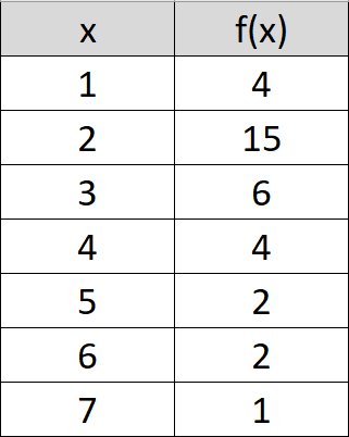
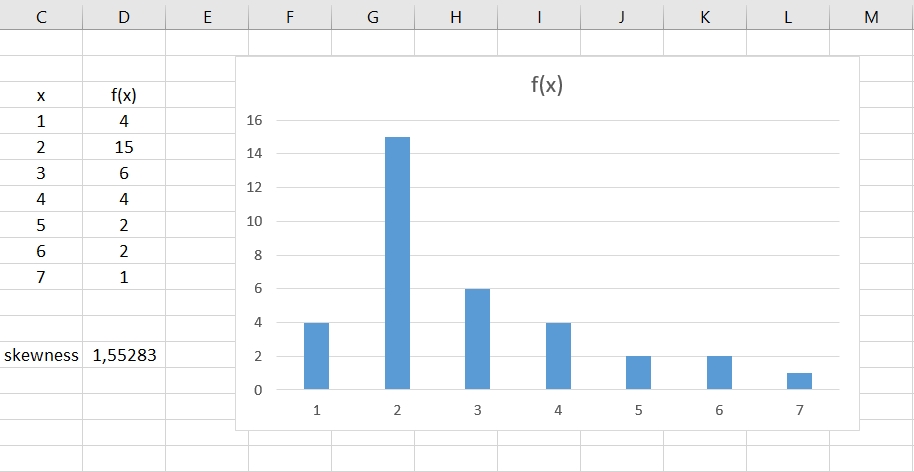
Article_Skewness_Figure_4 — Table of values

We insert the table in a spreadsheet in cells C3:D10 and applying the function in cell D13

SKEW.P(D4:D10)

we obtain the value 1.55283 as in the following figure.

Conclusion

The purpose of data collection is to analyze the data in order to make evaluations and, on the basis of these, make decisions. We have seen that often the only statistical analysis of the normal distribution of data is not sufficient to find the optimal strategy to apply, but it is necessary to deepen with the analysis of the shape of the distribution.

In this article Skewness is described and used through Microsoft Excel because it is the most popular and easy to use tool for everyone.

Another useful parameter to deepen our analysis is the Kurtosis that evaluates the height of the distribution of the data compared to the normal one. For those who want to deepen the usefulness of this, I invite you to read the related article “Kurtosis of data distribution”.

If you found this article useful and want to know about new articles, I invite you to sign up for my blog’s free newsletter J

Published with licenza CC BY-NC-ND 3.0 IT (Creative Common – Attribuzione – Non commerciale – Non opere derivate 3.0 Italia)

Subscribe Free Newsletter